Political Polling Part 1: Sampling
This post is part of a series on political polling. To start at the beginning, click here. The code used to generate the charts in this post can be found here.
The central idea that underpins all polling is the concept of statistical sampling, which may sound intimidating but for our purposes really boils down to two things:
- Surveying a small fraction of the total electorate can accurately reflect the preferences of the overall population.
- The polling results you get will be less precise the smaller your sample is.
That first point — whether or not your polls are predictive of actual election results — is something that I’ll cover in depth in future posts. But here I’ll talk about that second point: even the most accurate poll has uncertainty associated with it, just because you’ve only polled a tiny fraction of the full electorate.
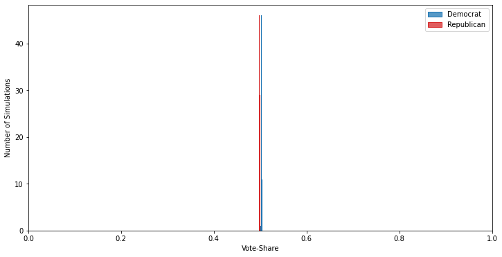
To illustrate this, let’s generate an example electorate. We’ll keep it simple: a single population of 1 million potential voters, with a slight preference for a Democratic candidate over a Republican, 50.2%–49.8%. Additionally, each person in this electorate has a 70% chance of actually voting in the election. 500 simulations of an election with these parameters look like this:
Zooming in just to the region around the simulation results shows that there is actually a distribution of outcomes:
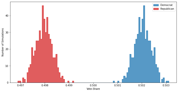
The vote margin varies due to sampling randomness, as in each simulation — like in reality — every voter has a less than 100% chance of actually voting. But with a million potential voters the electorate this distribution is really small: about 0.1% on either side of the actual result. Now let’s run five polls, each of 1000 random members of this electorate, and record the results:
| Poll | Democrat | Republican |
|---|---|---|
| 1 | 0.507 | 0.493 |
| 2 | 0.533 | 0.467 |
| 3 | 0.494 | 0.506 |
| 4 | 0.473 | 0.527 |
| 5 | 0.489 | 0.511 |
We know from how we set up the simulation that the Democrat is going to win the election with a margin of about 0.4%, and yet of these five polls the Republican is ahead in three of them, in one case by over 5%1. What gives?
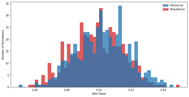
Well, it’s that sampling randomness again, only this time it’s a much larger effect because our sample is so small2. This is where poll aggregators like 538 or RealClearPolitics come into play: since individual polls have this significant intrinsic variation, it’s necessary to look at multiple polls in order to get an accurate picture of the race. For example, if instead of looking at only five polls we look at 500, it becomes totally clear that the race is essentially a tossup:
The silver lining about sampling uncertainty is that it’s well understood for statistical problems like political polling, and as such is fairly easy to estimate: this is what the uncertainties (sometimes reported as “confidence intervals”) predominantly are.
This is not the only source of uncertainty or error in polling, however, and unfortunately other issues can bias polling results in ways that are much harder to compensate for. I’ll dig into those in upcoming posts.
-
If you look closely you’ll notice there’s also a poll in this sample where the Democrat is the one winning by more than 5%, but I focused on the polls with the Republican in the lead since the public cares way more about polling errors that suggest the wrong winner. ↩
-
If you’re having trouble with the concept of smaller samples producing less precise results, think about what would happen in the extreme case where we polled just two people. While, in a close election like this, most polls would show a 50-50 split in the vote, a fair few would happen to have polled two Democratic or Republican voters just by chance and show 100% of the vote going to one candidate. This is similar to flipping a coin several times — sometimes you’ll get 10 heads in a row, but that doesn’t mean the coin isn’t fair. ↩